A Practical Guide for Programmers

The Quiet Revolution: How Semantic Search Is Rewriting the Rules of Data Retrieval

For thirty years, we searched by matching words. Now machines understand what we mean. Here is how it works — and how to build it yourself.

Technical Deep Dive  ·  18 min read  ·  Python, SQL & Vector Databases

Chapter One

The Librarian Who Couldn’t Understand You

Imagine walking into the greatest library ever built. Every book humanity has ever written lines the shelves. You approach the librarian and say, “I need something about overcoming failure in business.” The librarian stares at you, then walks to the card catalog and searches for the exact words: overcoming, failure, business. She returns with three results — one about business licenses containing the word “failure” in a liability clause, another about overcoming allergies at business lunches, and a pamphlet about overcoming fear of failure in youth basketball.

The book you actually needed — Shoe Dog by Phil Knight, a memoir about building Nike through decades of near-bankruptcy, doubt, and relentless perseverance — sits untouched on the shelf. It never used the word “failure” in its description. The librarian matched your words but missed your meaning.

This is the world we built with keyword search. For three decades, from early SQL LIKE clauses to Elasticsearch and Apache Solr, our search infrastructure has been spectacularly good at one thing — finding exact matches — and spectacularly bad at the thing humans actually need: understanding intent.

Semantic search changes this. It doesn’t match words. It matches meaning. And for programmers willing to learn its mechanics, it opens a category of applications that were simply impossible before: support systems that understand customer problems described in natural language, legal discovery tools that find relevant precedent across different phrasings, medical research platforms that surface related studies regardless of terminology.

This isn’t a future technology. It’s production-ready today. And you can build it with tools you largely already know.

Chapter Two

What Semantic Search Actually Is

At its core, semantic search replaces the question “Do these strings match?” with “Do these ideas live near each other in meaning-space?”

To accomplish this, every piece of text — every document, every query, every sentence — is transformed into a vector embedding: a dense array of floating-point numbers (typically 384 to 3,072 dimensions) that represents the meaning of that text in a high-dimensional geometric space.

Think of it this way

If traditional search is a dictionary lookup — rigid, literal, binary — then semantic search is a conversation with someone who has read everything. You describe what you need in your own words, and they reach for the right thing, even if you describe it differently than the author did.

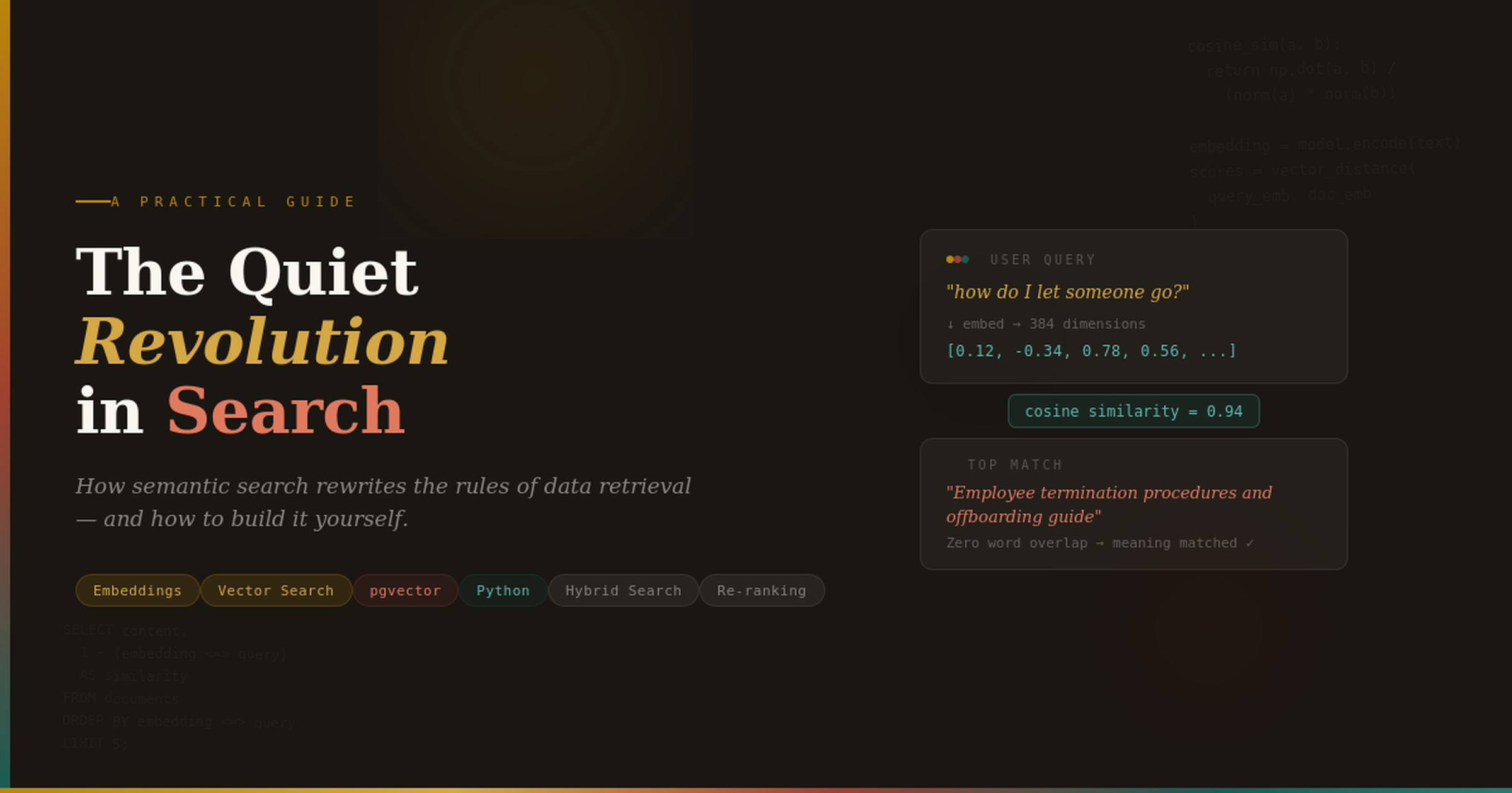
Two sentences that mean similar things will produce vectors that are geometrically close together, even if they share zero words. “How to terminate an employee” and “Process for letting a team member go” are far apart lexically but nearly identical semantically. A cosine similarity computation between their embeddings would return a score near 1.0.

Keyword Search

Lexical Matching

Finds documents containing the exact query terms. Fast, precise for known terms, but blind to synonyms, context, and user intent.

Semantic Search

Meaning Matching

Finds documents whose meaning is closest to the query’s meaning. Handles paraphrases, synonyms, and conceptual similarity without explicit rules.

Dimension	Keyword Search	Semantic Search
Query	“employee termination process”	“how do I let someone go?”
Matching	Exact token overlap (TF-IDF, BM25)	Vector distance in embedding space
Synonyms	Requires manual synonym lists	Handled automatically by embeddings
Precision	High when terms are specific	High when meaning is clear
Setup Cost	Low — inverted index	Moderate — embedding model + vector index
Best For	SKU lookups, exact phrases, IDs	Natural language queries, discovery, Q&A

The most powerful search systems of the next decade won’t be the ones that index the most data. They’ll be the ones that understand what the user actually needs.

Chapter Three

The Machinery of Meaning: How Embeddings Work

An embedding model — a neural network trained on billions of text pairs — reads a piece of text and outputs a fixed-length array of numbers. These numbers aren’t random. They encode relationships. Words that co-occur in similar contexts produce similar vectors. Sentences that express similar ideas cluster together in the high-dimensional space.

The practical consequence is that you can measure the similarity between any two pieces of text by computing the cosine similarity between their vectors — essentially measuring the angle between two arrows in a 768-dimensional space. An angle of 0° means identical meaning. An angle of 90° means completely unrelated.

Choosing an Embedding Model

Not all embedding models are equal. Your choice depends on the trade-off between quality, speed, and cost. Here is the current landscape that matters for production use:

Model	Dimensions	Best For
all-MiniLM-L6-v2	384	Prototyping, low-latency apps. Free, runs locally. Solid baseline.
text-embedding-3-small	1,536	Production workloads. Best price/performance from OpenAI.
text-embedding-3-large	3,072	Maximum quality. Legal, medical, and nuanced domains.
voyage-3	1,024	Code search and technical documentation. Top MTEB scores.
Cohere embed-v3	1,024	Multilingual applications. 100+ languages.

Let us see this in action. The following Python snippet generates embeddings using the open-source sentence-transformers library — no API key required:

Python

from sentence_transformers import SentenceTransformer
import numpy as np

# Load model (downloads once, ~90MB)
model = SentenceTransformer('all-MiniLM-L6-v2')

# Your documents
documents = [
    "How to handle employee termination procedures",
    "Process for letting a team member go gracefully",
    "Best practices for onboarding new hires",
    "Guide to firing underperforming staff",
    "Setting up a new development environment",
]

# Generate embeddings — each becomes a 384-dim vector
doc_embeddings = model.encode(documents)

# The user's query
query = "how do I let someone go from the company?"
query_embedding = model.encode([query])[0]

# Compute cosine similarity between query and all documents
def cosine_sim(a, b):
    return np.dot(a, b) / (np.linalg.norm(a) * np.linalg.norm(b))

scores = [(doc, cosine_sim(query_embedding, emb))
          for doc, emb in zip(documents, doc_embeddings)]

# Sort by relevance
for doc, score in sorted(scores, key=lambda x: x[1], reverse=True):
    print(f"{score:.3f} → {doc}")

Run this and the output will surprise you. Despite sharing almost no words with the query, “Process for letting a team member go gracefully” and “Guide to firing underperforming staff” will rank highest. “Setting up a new development environment” — which shares the word pattern of “setting up” — will rank dead last. The model understood meaning, not words.

Chapter Four

Building a Production Semantic Search System

Understanding the concept is the easy part. Shipping it to production requires thinking about three engineering challenges: how to generate embeddings efficiently, how to store and index them for fast retrieval, and how to query them in a way that scales. Let us work through each.

Semantic Search Pipeline

Raw Text
Documents, records

→

Chunking
Split into passages

→

Embedding
Text → Vectors

→

Vector Store
Index & persist

→

Query & Rank
Similarity search

Every semantic search system follows this five-stage pipeline. The key engineering decisions happen at stages 2, 3, and 4.

Chunk Your Documents Intelligently

Embedding models have token limits (typically 256–512 tokens for optimal quality). Long documents must be split into chunks. But how you split them matters enormously — poor chunking is the number one cause of bad search results.

Python

from langchain.text_splitter import RecursiveCharacterTextSplitter

splitter = RecursiveCharacterTextSplitter(
    chunk_size=500,          # Characters per chunk
    chunk_overlap=50,        # Overlap to preserve context
    separators=["\n\n", "\n", ". ", " "]  # Split at natural boundaries
)

raw_text = open("company_handbook.txt").read()
chunks = splitter.split_text(raw_text)

print(f"Split into {len(chunks)} chunks")
print(f"Average chunk size: {sum(len(c) for c in chunks) // len(chunks)} chars")

The overlap parameter is critical. Without it, a sentence that straddles two chunks loses its meaning in both. With 50–100 characters of overlap, the same sentence appears intact in at least one chunk.

Store Vectors in a Purpose-Built Index

Once you have embeddings, you need somewhere to store them where similarity queries run in milliseconds, not minutes. Three serious options dominate the landscape today, each with a distinct use case:

• pgvector (PostgreSQL extension) — If you already run Postgres, add vector search with a single CREATE EXTENSION. Perfect for teams who don’t want another database to manage.
• Pinecone / Weaviate / Qdrant — Managed vector databases built for scale. Best when you have millions of vectors and need sub-10ms latency.
• Oracle 23ai / SQL Server — Enterprise databases with native vector support. Ideal when your vectors must coexist with relational data under the same security and governance model.

Here’s the pgvector approach — the fastest path from zero to production for most teams:

SQL — PostgreSQL + pgvector

-- Enable the extension
CREATE EXTENSION IF NOT EXISTS vector;

-- Create a table with a vector column
CREATE TABLE documents (
    id          SERIAL PRIMARY KEY,
    title       TEXT,
    content     TEXT,
    chunk_index INTEGER,
    embedding   vector(384),   -- Matches MiniLM output
    created_at  TIMESTAMPTZ DEFAULT NOW()
);

-- Create an IVFFlat index for fast similarity search
CREATE INDEX ON documents
USING ivfflat (embedding vector_cosine_ops)
WITH (lists = 100);  -- Tune: sqrt(num_rows) is a good starting point

-- Query: find the 5 most similar documents
SELECT title, content,
       1 - (embedding <=> '[0.12, -0.34, ...]'::vector) AS similarity
FROM   documents
ORDER BY embedding <=> '[0.12, -0.34, ...]'::vector
LIMIT  5;

The <=> operator computes cosine distance. The IVFFlat index partitions the vector space into clusters so the database only scans the most relevant partition during queries — analogous to how a B-tree index prunes the search space for range queries.

Build the Complete Ingestion Pipeline

With chunking, embedding, and storage in place, here’s a complete Python pipeline that ingests documents into your semantic search engine:

Python

import psycopg2
from sentence_transformers import SentenceTransformer
from langchain.text_splitter import RecursiveCharacterTextSplitter

# Initialize
model = SentenceTransformer('all-MiniLM-L6-v2')
splitter = RecursiveCharacterTextSplitter(chunk_size=500, chunk_overlap=50)
conn = psycopg2.connect("dbname=semantic_search user=postgres")

def ingest_document(title: str, text: str):
    """Chunk, embed, and store a document."""
    chunks = splitter.split_text(text)
    embeddings = model.encode(chunks)

    with conn.cursor() as cur:
        for i, (chunk, emb) in enumerate(zip(chunks, embeddings)):
            cur.execute(
                """INSERT INTO documents (title, content, chunk_index, embedding)
                   VALUES (%s, %s, %s, %s)""",
                (title, chunk, i, emb.tolist())
            )
    conn.commit()

def search(query: str, top_k: int = 5) -> list:
    """Semantic search: find the most relevant chunks."""
    query_emb = model.encode([query])[0].tolist()

    with conn.cursor() as cur:
        cur.execute("""
            SELECT title, content,
                   1 - (embedding <=> %s::vector) AS similarity
            FROM   documents
            ORDER BY embedding <=> %s::vector
            LIMIT  %s
        """, (str(query_emb), str(query_emb), top_k))
        return cur.fetchall()

# Usage
ingest_document("Employee Handbook", open("handbook.txt").read())

results = search("how do I request time off?")
for title, content, score in results:
    print(f"\n[{score:.3f}] {title}")
    print(f"{content[:200]}...")

Add Hybrid Search for Best-of-Both-Worlds

In practice, the most effective systems don’t choose between keyword and semantic search. They combine both. This is called hybrid search, and it’s what powers the best production systems at companies like Notion, Stripe, and Shopify.

The principle is simple: run both a traditional full-text search and a semantic vector search, then fuse their results using a technique called Reciprocal Rank Fusion (RRF):

Python

def hybrid_search(query: str, top_k: int = 5, alpha: float = 0.7):
    """
    Combine semantic + keyword search with Reciprocal Rank Fusion.
    alpha controls the weight: 1.0 = pure semantic, 0.0 = pure keyword.
    """
    # Semantic results
    semantic_results = search_semantic(query, top_k=20)
    # Keyword results (e.g., PostgreSQL ts_rank)
    keyword_results = search_keyword(query, top_k=20)

    # Reciprocal Rank Fusion
    k = 60  # RRF constant — standard value
    fused_scores = {}

    for rank, (doc_id, _) in enumerate(semantic_results):
        fused_scores[doc_id] = fused_scores.get(doc_id, 0)
        fused_scores[doc_id] += alpha * (1 / (k + rank + 1))

    for rank, (doc_id, _) in enumerate(keyword_results):
        fused_scores[doc_id] = fused_scores.get(doc_id, 0)
        fused_scores[doc_id] += (1 - alpha) * (1 / (k + rank + 1))

    # Return top-K by fused score
    ranked = sorted(fused_scores.items(), key=lambda x: x[1], reverse=True)
    return ranked[:top_k]

The alpha parameter is your most important tuning knob. For natural language queries (“how do I set up SSO?”), weight semantic search heavily (alpha = 0.8). For specific lookups (“error code ERR-4021”), weight keywords heavily (alpha = 0.2). Many production systems adjust alpha dynamically based on query characteristics.

Chapter Five

The Art of Tuning: From Good to Remarkable

A basic semantic search implementation will impress you. A well-tuned one will impress your users. The difference lives in four decisions that most tutorials gloss over.

Chunk Size: The Single Most Impactful Parameter

If your chunks are too small (under 200 characters), the embedding captures so little context that “reset my password” and “reset the database” look similar — both involve “reset.” If your chunks are too large (over 2,000 characters), the embedding becomes a blurry average of multiple ideas, and precision drops. The sweet spot for most English-language content is 400–800 characters with 50–100 characters of overlap.

Metadata Filtering: Narrow Before You Search

Vector similarity alone isn’t enough for real applications. A support agent searching for billing issues doesn’t need results from engineering docs. Use metadata filters to constrain the search space before computing vector distances:

SQL

-- Filter FIRST, then rank by semantic similarity
SELECT title, content,
       1 - (embedding <=> $query_vector::vector) AS similarity
FROM   documents
WHERE  department = 'billing'
  AND  created_at > '2024-01-01'
ORDER BY embedding <=> $query_vector::vector
LIMIT  5;

Re-ranking: The Quality Multiplier

Fast embedding models (like MiniLM) are excellent at narrowing millions of documents to the top 50 candidates. But for the final ranking — deciding which 5 results the user actually sees — a more powerful cross-encoder re-ranker can dramatically improve precision:

Python

from sentence_transformers import CrossEncoder

# Cross-encoder scores query-document PAIRS (more accurate, slower)
reranker = CrossEncoder('cross-encoder/ms-marco-MiniLM-L-6-v2')

def search_with_reranking(query, top_k=5):
    # Stage 1: Fast retrieval — get 50 candidates
    candidates = search_semantic(query, top_k=50)

    # Stage 2: Re-rank with cross-encoder
    pairs = [(query, doc['content']) for doc in candidates]
    scores = reranker.predict(pairs)

    # Sort by re-ranked score
    ranked = sorted(zip(candidates, scores), key=lambda x: x[1], reverse=True)
    return ranked[:top_k]

This two-stage approach — fast retrieval followed by precise re-ranking — is the architecture behind virtually every high-quality search system in production today. It is the same principle as a database optimizer using an index scan to find candidate rows, then applying expensive predicates to filter the final result set.

Evaluation: How to Know If It’s Working

Build a test set of 50–100 query/expected-result pairs from real user queries. Measure Recall@5 (does the correct document appear in the top 5 results?) and MRR (Mean Reciprocal Rank — how high does the correct result rank?). If Recall@5 is below 0.8, your chunking strategy or embedding model needs work before anything else.

Chapter Six

Where This Changes Everything

Semantic search is not a solution looking for a problem. It is the missing layer in applications that have struggled with natural language input for decades. Here are four implementations that are transforming their respective domains right now.

• Customer Support (RAG-Powered Q&A): Retrieve relevant knowledge base articles using semantic search, pass them as context to an LLM, and generate accurate answers in natural language. This is Retrieval-Augmented Generation — and semantic search is its engine.
• Legal Discovery: A lawyer searching for precedent about “breach of fiduciary duty in mergers” finds cases filed under “director negligence in acquisition contexts” — same concept, zero word overlap.
• Internal Knowledge Management: Enterprise wikis and Confluence pages become searchable by what they’re about, not just what they contain. Teams finally find that design decision document from 18 months ago.
• E-Commerce Product Search: A customer searching for “something to keep my coffee hot at my desk” finds the insulated travel mug — not just products with “hot” and “coffee” in the title.

Chapter Seven

The Road Ahead — And Why You Should Start Now

We are in the early innings of a fundamental shift in how software understands human language. The embedding models are getting better and cheaper every quarter. The vector databases are maturing rapidly. And most importantly, users are beginning to expect that when they describe what they need in plain language, the software should understand.

If you are a programmer who has spent years working with traditional search — Elasticsearch, Solr, SQL full-text indexes — you are not obsolete. You are uniquely prepared. You understand inverted indexes, you understand relevance scoring, you understand the importance of recall and precision. Semantic search doesn’t replace that knowledge. It builds on it.

The most effective search systems of the next decade will be hybrid systems — keyword search for precision, semantic search for understanding, and re-ranking models for quality. The engineers who can architect these systems, who understand both the information retrieval fundamentals and the new vector-based techniques, will be the ones building the products people actually love to use.

Start small. Take a corpus you know well — your company’s help docs, your personal notes, a collection of papers in your field. Chunk it, embed it, index it, and query it. The moment you search for a concept in your own words and the system returns exactly what you needed — even though you described it nothing like the author did — something clicks. You realize that search has been broken your whole career, and now it’s not.

That’s not hype. That’s an engineering fact. And you’re the one who gets to build it.

Key Takeaways

• Semantic search matches meaning, not words. Text is converted to vector embeddings — numerical representations that capture semantic relationships — and similarity is measured as geometric distance.
• The core pipeline is five stages: chunk documents, generate embeddings, store in a vector index, query by embedding the user’s question, and rank by cosine similarity.
• pgvector makes this accessible today. A single PostgreSQL extension gives you vector storage and similarity search alongside your existing relational data — no new infrastructure required.
• Hybrid search (keyword + semantic) outperforms either alone. Use Reciprocal Rank Fusion to combine both approaches, with alpha-weighting tuned to your query patterns.
• Chunk size and re-ranking are your highest-leverage tuning parameters. Get chunk size right (400–800 chars) and add a cross-encoder re-ranker to move from good to remarkable.
• Start with all-MiniLM-L6-v2 for prototyping — it’s free, runs locally, and produces surprisingly strong results. Upgrade to OpenAI or Cohere embeddings when you need production-grade quality or multilingual support.

Continue the Series

II

From Search to Answers: Building RAG Systems That Don’t Hallucinate

Connect your semantic search engine to an LLM and build a question-answering system with citations, confidence scoring, and graceful “I don’t know” responses.

III

Multimodal Search: When Your Data Isn’t Just Text

Extend semantic search to images, PDFs, code repositories, and audio transcripts using CLIP, ColPali, and unified embedding spaces.

IV

Scaling to 100 Million Vectors: Architecture Decisions That Matter

Sharding strategies, quantization techniques, HNSW vs. IVF index selection, and the real-world cost of vector search at enterprise scale.

◆ ◆ ◆

We spent thirty years teaching computers to read words. We’re finally teaching them to understand sentences.